The Hidden Math Behind Every Oscillating System You Encounter"
A mass on a spring. A child on a swing. An electrical circuit humming along. These all share something fundamental: they oscillate, and sometimes that oscillation gets complicated when external forces enter the picture.
The Problem With External Forces
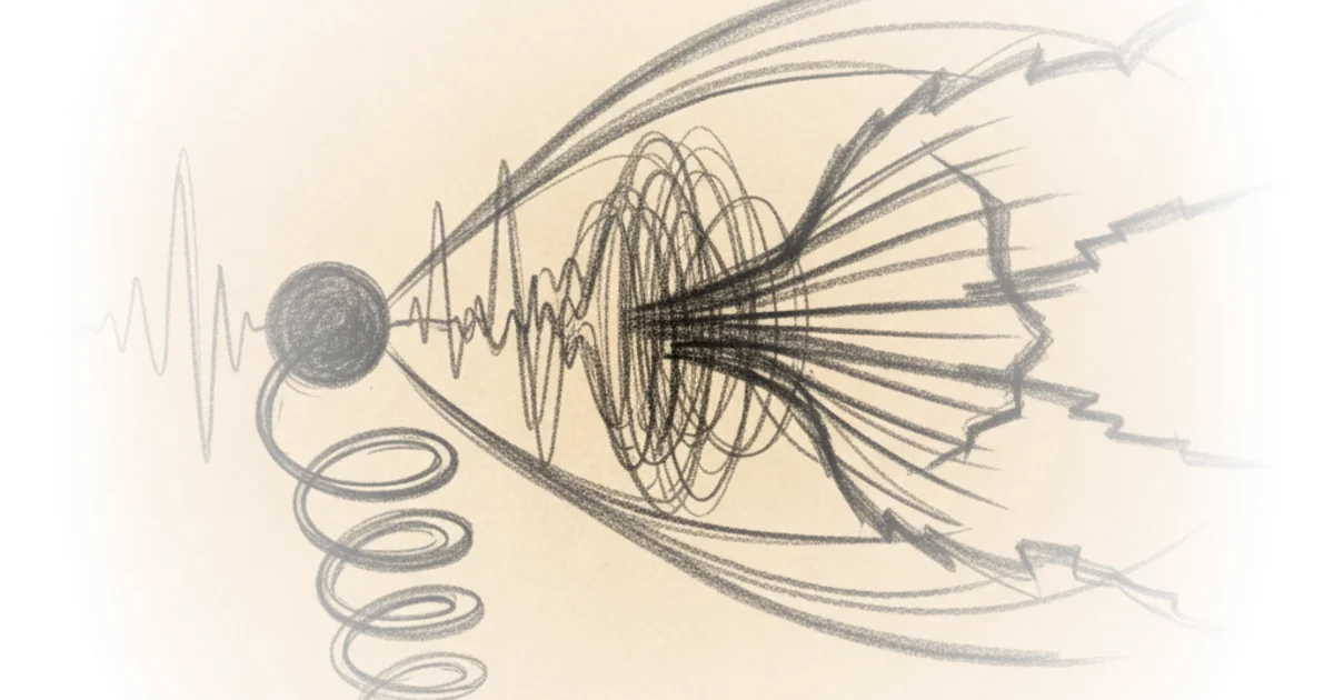
Consider a simple system: a mass attached to a spring, pulled toward its center position by a force proportional to how far it is from that center. Add some damping to slow the motion down over time. This is the classic harmonic oscillator.
Now introduce an external force pushing the mass back and forth like wind gusts, oscillating according to cosine function. The frequency of this external force has nothing to do with the spring's natural resonant frequency.
The behavior is fascinating. Initially, things look chaotic. The oscillation gets stronger and weaker in unpredictable ways before eventually settling into a rhythm. Why does this happen? How long until it stabilizes? And how big will those final oscillations be?
This is where Laplace transforms become invaluable.
What Is the S-Plane?
The Laplace transform takes a function of time and converts it into a new function whose input is a complex number s—engineers call this the s-plane. Each point in that plane encodes an entire exponential function like e^(s*t).
Big imaginary values of s correspond to functions with more oscillation. Negative real parts reflect decay toward zero. Positive real parts reflect growth or instability.
The reason this matters: many functions in nature can be broken down into exponential pieces. The Laplace transform acts as a machine that exposes exactly how that breakdown looks.
Two Properties Worth Remembering
First, linearity. If you have a scaled sum of functions and apply the transform to each individually, taking that same scaled sum of the results gives you the same answer. This means complex functions can be decomposed into simpler pieces.
Second, exponential behavior. When pumping in an expression like e^(a*t), it transforms into 1/(s-a)—an expression with a pole above the value a in the s-plane.
These properties together give engineers a qualitative sense of system dynamics. After finding a system's Laplace transform, they can look at where poles land: imaginary values indicate oscillation, negative real parts indicate decay toward zero, positive real parts indicate instability or explosion.
From Differential Equations to Algebra
The most powerful property involves derivatives. When taking the Laplace transform of a derivative, it transforms into multiplication by s in the s-domain—plus subtracting off initial conditions.
This is why it's so useful: differential equations turn into polynomials, and polynomials are far easier to work with algebraically than derivatives.
Walking Through an Example
Let's apply this to that mass-spring system with external oscillating force. The equation includes terms for position, velocity, damping, and the cosine forcing function.
When taking the Laplace transform of all terms, the transform of each derivative becomes s multiplied by its transformed variable minus initial conditions. Substituting through gives a polynomial with constants from the original equation.
If we assume both initial position and velocity are zero—starting completely stationary—that simplifies things considerably. The left side transforms into that polynomial mirror image: s² times the transformed variable, plus mu*s times transformed variable, plus k times transformed variable. This is exactly why the tool works so well: differential expressions turn into polynomials.
The right side requires taking the Laplace transform of cosine, which creates two poles—one at ωi and one at negative ωi—reflecting oscillation with frequency ω.
Now we have an expression describing the Laplace transform of our solution. From here, inverting the transform reveals the original function in the time domain.
What Poles Reveal
Just by seeing this transformed version, you gain intuition about system dynamics. The key question is: where are all the poles?
The polynomial part creates two roots—typically with negative real parts and an imaginary component assuming damping isn't too large. When poles land like that, what's revealed is oscillation with decay: the unforced oscillator's behavior, matching the spring's natural resonant frequency.
The other poles come from ω and negative ω—the external cosine force. These correspond to a tendency to oscillate in sync with that external force.
If you push a child on a swing with a frequency that doesn't match their natural frequency, what ultimately happens? They oscillate in your frequency, not the swing's. The same principle applies here: dominant behavior is oscillation matching the external forcing function.
Counterpoints
A critic might note this approach has limitations for truly nonlinear systems—the transform only handles linear differential equations directly. Also, the initial conditions assumption simplifies things considerably; general solutions require keeping those constants around.
Bottom Line
The strongest argument for Laplace transforms is their ability to convert impossible differential equations into solvable algebra while simultaneously revealing system behavior through pole locations. The vulnerability: this requires assuming clean initial conditions and works best on linear systems. For anyone analyzing oscillators, circuits, or control systems, the transform isn't just a mathematical trick—it's a window into understanding exactly how dynamic systems behave before solving them.